2. Geography chapter of Regrarians eHandbook released

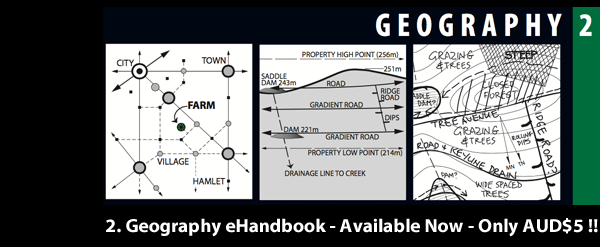
After a very long gestation, the Regrarians Handbook team were able to finally get the 2.Geography chapter out today. We produced some 12 versions of this quite detailed chapter and many, many iterations and background maps and so on — particularly for the two Keyline sections.

We took a very different approach with the Keyline sections — at our planning meeting for this chapter, Andrew Jeeves, Owen Hablutzel and myself nutted out the process by which we’d undertake these sections. I wanted to have a ‘whole of landscape’ approach to explaining Keyline Geography and Geometry and apply it to landscapes that actually exist. For this we needed a map!

Andrew’s in the local country fire brigade and so we went up the road to the shed and I pulled out of the map rack the 1:25000 series ‘Bega’ mapsheet. We opened it up and went straight to a catchment and landscape that ticked the boxes. We then went back to Andrew’s place and took a closer look. We all agreed that this catchment and landscape had what was needed. This whole process took all of 10 mins!

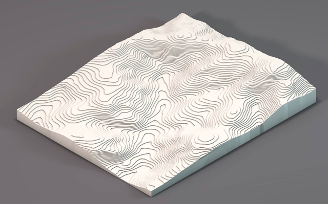
Next we needed to create a digital elevation model so that this landscape would come to life — that’s where our friend and colleague Georgi Pavlov of HUMA Design got to work. We found some 1 second DEM data and made 5 different zoom levels (‘A’ – ‘E’) of the chosen catchment and ‘home landscape’.

Credit: Georgi Pavlov (HUMA Design), Geoscience Australia

The ‘A’ landscape is of a whole catchment from ridge to the sea and covers approx. 35,000 ha (86,000 acres) — representing the understanding of the lower 4 orders of water flow (i.e Creek to Ocean – out of a total of 7). The ‘B’ landscape covers 14,700 ha (36,000 acres) and represents a smaller catchment, the level at which Primary Valleys, Secondary Valleys and Primary Ridges can start to be discerned. The ‘C’ landscape is around 1520 ha (2800 ha) and represents the size of some private landholdings in this particular area — it also is where we can start to identify Keypoints and Keylines more clearly. The ‘D’ landscape is 255 ha (630 acres) and this is our realistic version of a catchment enclosing the first 4 orders of water flow (i.e Sheet to Creek). This landscape is synonymous with Andrew Jeeves’ classic diagram, Fig 2.1 p.14 ‘Designing to Catch and Store Energy’, in Permaculture: A Designers’ Manual (Mollison, Tagari, 1988).

Credit: Georgi Pavlov (HUMA Design), Geoscience Australia

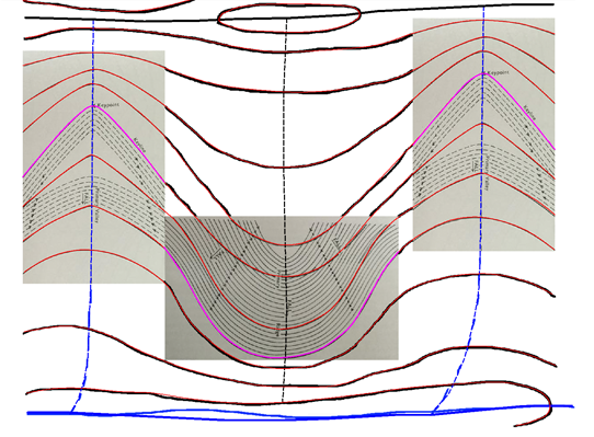
When it came to working on the Keyline Geometry section we had a number of goes at a few approaches using this ‘home landscape’. Reading through P.A. Yeomans, ‘The Challenge of Landscape’, the idea came to me to use some of the contour diagrams included in this book for a few reasons — one was to create an ‘interpretive lineage’ between the original work of P.A. Yeomans and our own, another was to continue to honour Mr. Yeomans genius, and finally it was because these maps were without any of the anomalies that are found in real landscapes that I decided we need to ‘start simple’ before heading off to some ‘real hills’!

Credit: Darren J Doherty, P.A. Yeomans

In literally hundreds of classes over the years I’ve been drawing a basic primary land unit landscape onto whiteboards and then drafting a series of comparitive guidelines over the top that represent the patterns of the equidistant grid-based rows, contour-based rows and Keyline-based rows. Every time I finished one I’d say, “I must do this digitally one day!”, and so with this Keyline Geometry section we started out with some rehashes of some of Mr. Yeomans work and then progressed through to a realistic application of the work onto the ‘E’ landscape — this being a 40 ha (100 acre) parcel.

Credit: Darren J Doherty, Georgi Pavlov (HUMA Design), Geoscience Australia

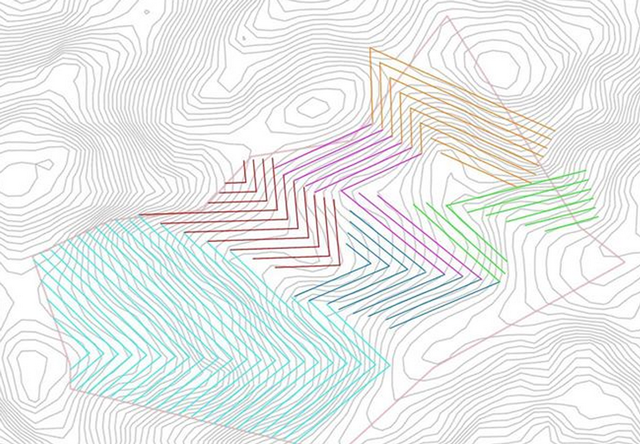
The ‘E’ landscape drafted above represents some of the geometric issues involved with applying Keyline Pattern Cultivation lines to a real landscape where primary valleys and ridges are don’t have the beautifully straight valley floor and ridge divide centrelines. Accordingly its tough to get the geometry as you would like. The secondary issue is that of the gradient of some of these lines — some end up with quite a fall on them and so in our finished detail we’ll often re-establish a new pattern to accomodate this issue.

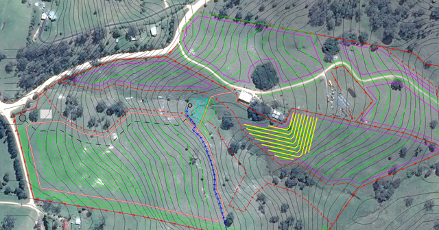
Credit: Darren J Doherty, Georgi Pavlov (HUMA Design), Geoscience Australia, GoogleEarth

The diagram above is my MapInfo-based rendition that Andrew turned into Fig. 2.35: Realistic application of Keyline geometry to agroforestry development and general farm layout at ‘Home Farm’ in the Geography chapter. You can see the way in which we’ve reduced gradients, not included the main primary valley in the patterning and so. This represents the shift from the theoretical to the realistic application of many of these Keyline patterns.

Otherwise in the Geography chapter, as throughout the rest of the book, we’ve tried to combine the functions of the ‘how-to’ and also of the best practice. We’ve subordinated the sections into categories and these flow according to the order with which one would approach a project. We’ve also boldly attempted to establish some standard languages within this sector, and we expect that users of our program will start to apply some of the conventions and language used.

As is our way, we’ve scoured the planet for the most broadly applicable tools, techniques and approaches to hope that these resonate widely with the Regrarians Handbook’s growing audience.

Now onto 3. Water!